From our 2012 Repost: Dreamtime Finance (and the Kelly Criterion):
We have a couple good posts on Mr. Thorpe, links below.
First though a short diversion:
Repost: Dreamtime Finance (and the Kelly Criterion)
First posted June 13, 2011.And today's link, from economist Lars P. Syll's blog:
Original post:
I've been meaning to write about Kelly for a couple years and keep forgetting. Today I forget no more.
In probability theory the Kelly Criterion is a bet sizing technique used when the player has a quantifiable edge.
(When there is no edge the optimal bet size is $0.00)
The criterion will deliver the fastest growth rate balanced by reduced risk of ruin.
You can grow your pile faster but you increase the risk of ending up broke should you, for example bet 100% of your net worth in a situation where you have anything less than a 100% chance of winning.
The criterion says bet roughly your advantage as a percentage of your current bankroll divided by the variance of the game/market/sports book etc..
Variance is the standard deviation of the game squared. In blackjack the s.d. is 1.15 so the square is 1.3225.
As blackjack is played in the U.S. the most a card counter can hope for is a 1/2% to 1% average advantage with much of that average accruing from the fact that you can get up from a negative table.
Divide by 1.3225 and you've got your bet size.
It's a tough way to grind out a living but hopefully this exercise will stop you from pulling a Leeson, betting all of Barings money and destroying the 233 year old bank.
I'll be back with more later this week.In the meantime here's a UWash paper with the formulas for equities investment....MORE
Expected utility, the Kelly criterion, and transmogrification of truth
...On a more economic-theoretical level, information theory — and especially the so called the Kelly criterion — also highlights the problems concerning the neoclassical theory of expected utility.
Suppose I want to play a game. Let’s say we are tossing a coin. If heads comes up, I win a dollar, and if tails comes up, I lose a dollar. Suppose further that I believe I know that the coin is asymmetrical and that the probability of getting heads (p) is greater than 50% – say 60% (0.6) – while the bookmaker assumes that the coin is totally symmetric. How much of my bankroll (T) should I optimally invest in this game?
A strict neoclassical utility-maximizing economist would suggest that my goal should be to maximize the expected value of my bankroll (wealth), and according to this view, I ought to bet my entire bankroll.
Does that sound rational? Most people would answer no to that question. The risk of losing is so high, that I already after few games played — the expected time until my first loss arises is 1/(1-p), which in this case is equal to 2.5 — with a high likelihood would be losing and thereby become bankrupt. The expected-value maximizing economist does not seem to have a particularly attractive approach.
So what’s the alternative? One possibility is to apply the so-called Kelly criterion — after the American physicist and information theorist John L. Kelly, who in the article A New Interpretation of Information Rate (1956) suggested this criterion for how to optimize the size of the bet — under which the optimum is to invest a specific fraction (x) of wealth (T) in each game. How do we arrive at this fraction?
When I win, I have (1 + x) times as much as before, and when I lose (1 – x) times as much. After n rounds, when I have won v times and lost n – v times, my new bankroll (W) is
(1) W = (1 + x)v(1 – x)n – v T
[A technical note: The bets used in these calculations are of the "quotient form" (Q), where you typically keep your bet money until the game is over, and a fortiori, in the win/lose expression it's not included that you get back what you bet when you win. If you prefer to think of odds calculations in the "decimal form" (D), where the bet money typically is considered lost when the game starts, you have to transform the calculations according to Q = D - 1.]
The bankroll increases multiplicatively — “compound interest” — and the long-term average growth rate for my wealth can then be easily calculated by taking the logarithms of (1), which gives
(2) log (W/ T) = v log (1 + x) + (n – v) log (1 – x).
If we divide both sides by n we get
(3) [log (W / T)] / n = [v log (1 + x) + (n - v) log (1 - x)] / n
The left hand side now represents the average growth rate (g) in each game. On the right hand side the ratio v/n is equal to the percentage of bets that I won, and when n is large, this fraction will be close to p. Similarly, (n – v)/n is close to (1 – p). When the number of bets is large, the average growth rate is
(4) g = p log (1 + x) + (1 – p) log (1 – x).
Now we can easily determine the value of x that maximizes g:
(5) d [p log (1 + x) + (1 - p) log (1 - x)]/d x = p/(1 + x) – (1 – p)/(1 – x) =>
p/(1 + x) – (1 – p)/(1 – x) = 0 =>
(6) x = p – (1 – p)
Since p is the probability that I will win, and (1 – p) is the probability that I will lose, the Kelly strategy says that to optimize the growth rate of your bankroll (wealth) you should invest a fraction of the bankroll equal to the difference of the likelihood that you will win or lose. In our example, this means that I have in each game to bet the fraction of x = 0.6 – (1 – 0.6) ≈ 0.2 — that is, 20% of my bankroll. Alternatively, we see that the Kelly criterion implies that we have to choose x so that E[log(1+x)] — which equals p log (1 + x) + (1 – p) log (1 – x) — is maximized. Plotting E[log(1+x)] as a function of x we see that the value maximizing the function is o.2:


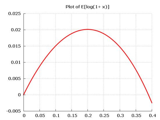
The optimal average growth rate becomesPossibly also of interest: "How did Ed Thorp Win in Blackjack and the Stock Market?" which includes and expands on the above and has a variation of the chart:
(7) 0.6 log (1.2) + 0.4 log (0.8) ≈ 0.02.
If I bet 20% of my wealth in tossing the coin, I will after 10 games on average have 1.0210 times more than when I started (≈ 1.22)....MORE
